MLとIntegratedMLでCovid-19のICU入室予測を実行する(パート1)
キーワード: IRIS、IntegratedML、機械学習、Covid-19、Kaggle
目的
最近、Covid-19患者がICU(集中治療室)に入室するかどうかを予測するKaggleデータセットがあることに気づきました。 231列のバイタルサインや観測で構成される1925件の遭遇記録が含まれる表計算シートで、最後の「ICU」列では「Yes」を示す1と「No」を示す0が使用されています。 既知のデータに基づいて、患者がICUに入室するかどうかを予測することがタスクです。
このデータセットは、「従来型ML」タスクと呼ばれるものの良い例のようです。 データ量は適切で、品質も比較的適切なようです。 IntegratedMLデモキットに直接適用できる可能性が高いようなのですが、通常のMLパイプラインと潜在的なIntegratedMLアプローチに基づいて簡易テストを行うには、どのようなアプローチが最も単純なのでしょうか。
範囲
次のような通常のMLステップを簡単に実行します。
- データのEDA(探索的データ分析)
- 特徴量の選択
- モデルの選択
- グリッド検索によるモデルパラメーターのチューニング
上記との比較で、次を実行します。
- SQLを介したIntegratedMLアプローチ
Docker-composeなどを使用して、AWS Ubuntu 16.04サーバーで実行します。
環境
integredML-demo-templateのDocker環境を再利用します。
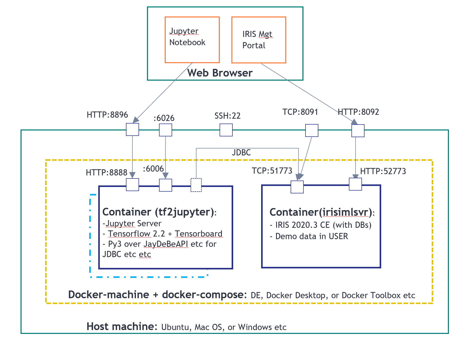
以下のノートブックファイルは「tf2jupyter」で実行しており、IRISとIntegratedMLは「irismlsrv」で実行しています。 Docker-composeはAWS Ubuntu 16.04で実行します。
データとタスク
このデータセットには、385人の患者から収集した1925件のレコードが含まれます。各患者にはちょうど5つの遭遇レコードがあります。 231列のうちの1つの列は、このトレーニングと予測のターゲットである「ICU」で、残りの230列は入力として使用することが可能です。 ICUは1または0のバイナリー値です。 カテゴリカル文字列(データフレームでは「オブジェクト」として表されます)のような2つの列を除くと、すべては数値データです。
import numpy as np
import pandas as pd
from sklearn.impute import SimpleImputer
import matplotlib.pyplot as plt
from sklearn.linear_model import LogisticRegression
from sklearn.model_selection import train_test_split
from sklearn.metrics import classification_report, roc_auc_score, roc_curve
import seaborn as sns
sns.set(style="whitegrid")
import os
for dirname, _, filenames in os.walk('./input'):
for filename in filenames:
print(os.path.join(dirname, filename))
./input/datasets_605991_1272346_Kaggle_Sirio_Libanes_ICU_Prediction.xlsx
df = pd.read_excel("./input/datasets_605991_1272346_Kaggle_Sirio_Libanes_ICU_Prediction.xlsx")
df| PATIENT_VISIT_IDENTIFIER | AGE_ABOVE65 | AGE_PERCENTIL | GENDER | DISEASE GROUPING 1 | DISEASE GROUPING 2 | DISEASE GROUPING 3 | DISEASE GROUPING 4 | DISEASE GROUPING 5 | DISEASE GROUPING 6 | ... | TEMPERATURE_DIFF | OXYGEN_SATURATION_DIFF | BLOODPRESSURE_DIASTOLIC_DIFF_REL | BLOODPRESSURE_SISTOLIC_DIFF_REL | HEART_RATE_DIFF_REL | RESPIRATORY_RATE_DIFF_REL | TEMPERATURE_DIFF_REL | OXYGEN_SATURATION_DIFF_REL | WINDOW | ICU | 1 | 60th | 0.0 | 0.0 | 0.0 | 0.0 | 1.0 | 1.0 | ... | -1.000000 | -1.000000 | -1.000000 | -1.000000 | -1.000000 | -1.000000 | -1.000000 | -1.000000 | 0-2 |
|---|---|---|---|---|---|---|---|---|---|---|---|---|---|---|---|---|---|---|---|---|---|
| 1 | 1 | 60th | 0.0 | 0.0 | 0.0 | 0.0 | 1.0 | 1.0 | ... | -1.000000 | -1.000000 | -1.000000 | -1.000000 | -1.000000 | -1.000000 | -1.000000 | -1.000000 | 2-4 | |||
| 2 | 1 | 60th | 0.0 | 0.0 | 0.0 | 0.0 | 1.0 | 1.0 | ... | NaN | NaN | NaN | NaN | NaN | NaN | NaN | NaN | 4-6 | |||
| 3 | 1 | 60th | 0.0 | 0.0 | 0.0 | 0.0 | 1.0 | 1.0 | ... | -1.000000 | -1.000000 | NaN | NaN | NaN | NaN | -1.000000 | -1.000000 | 6-12 | |||
| 4 | 1 | 60th | 0.0 | 0.0 | 0.0 | 0.0 | 1.0 | 1.0 | ... | -0.238095 | -0.818182 | -0.389967 | 0.407558 | -0.230462 | 0.096774 | -0.242282 | -0.814433 | ABOVE_12 | 1 | ||
| ... | ... | ... | ... | ... | ... | ... | ... | ... | ... | ... | ... | ... | ... | ... | ... | ... | ... | ... | ... | ... | ... |
| 1920 | 384 | 50th | 1 | 0.0 | 0.0 | 0.0 | 0.0 | 0.0 | 0.0 | ... | -1.000000 | -1.000000 | -1.000000 | -1.000000 | -1.000000 | -1.000000 | -1.000000 | -1.000000 | 0-2 | ||
| 1921 | 384 | 50th | 1 | 0.0 | 0.0 | 0.0 | 0.0 | 0.0 | 0.0 | ... | -1.000000 | -1.000000 | -1.000000 | -1.000000 | -1.000000 | -1.000000 | -1.000000 | -1.000000 | 2-4 | ||
| 1922 | 384 | 50th | 1 | 0.0 | 0.0 | 0.0 | 0.0 | 0.0 | 0.0 | ... | -1.000000 | -1.000000 | -1.000000 | -1.000000 | -1.000000 | -1.000000 | -1.000000 | -1.000000 | 4-6 | ||
| 1923 | 384 | 50th | 1 | 0.0 | 0.0 | 0.0 | 0.0 | 0.0 | 0.0 | ... | -1.000000 | -1.000000 | -1.000000 | -1.000000 | -1.000000 | -1.000000 | -1.000000 | -1.000000 | 6-12 | ||
| 1924 | 384 | 50th | 1 | 0.0 | 0.0 | 1.0 | 0.0 | 0.0 | 0.0 | ... | -0.547619 | -0.838384 | -0.701863 | -0.585967 | -0.763868 | -0.612903 | -0.551337 | -0.835052 | ABOVE_12 |
1925 rows × 231 columns
df.dtypesPATIENT_VISIT_IDENTIFIER int64 AGE_ABOVE65 int64 AGE_PERCENTIL object GENDER int64 DISEASE GROUPING 1 float64 ...
RESPIRATORY_RATE_DIFF_REL float64 TEMPERATURE_DIFF_REL float64 OXYGEN_SATURATION_DIFF_REL float64 WINDOW object ICU int64 Length: 231, dtype: object
この問題とそのアプローチを組むには、確実にいくつかのオプションがあります。 最初に頭に浮かぶのは、これが「二項分類」の問題と考えられることです。 すべての1925件のレコードを、同じ患者のレコードであるかに関係なく、「ステートレス」の個別のレコードとして扱うことができます。 もちろん、ICUと他の値をすべて数値として扱うのであれば、「回帰」問題としても考えられるでしょう。
確かにほかのアプローチもあります。 たとえば、データセットに、患者ごとに異なる385件の短い「時系列」があるというように扱うこともできます。 セット全体をTrain/Val/Test用の385個の個別のセットに分解した場合は、CNNやLSTMなどのディープラーニングモデルを使って、個々の患者ごとに各セットに隠れた「症状の発展段階またはパターン」をキャプチャできるでしょうか? できるかもしれませんね。 それを行えば、データ拡張も適用して、様々な方法でテストデータを充実させることができるかもしれません。 これについては、この記事の対象外として別のトピックとしましょう。
この記事では、いわゆる「従来型ML」とIntegratedML(AutoML)アプローチのクイックランをテストします。
「従来型」MLアプローチとは
このデータセットは、いくつかの値が欠落していることを除き、ほとんどの実際のケースより比較的正規化されたものであるため、特徴量エンジニアリングの部分を省略して、直接列を特徴量として使用できる可能性があります。 では早速、特徴量の選択に進みましょう。
欠落しているデータを代入する
まず、すべての欠落している値が単純な代入で埋められていることを確認します。
df_cat = df.select_dtypes(include=['object'])
df_numeric = df.select_dtypes(exclude=['object'])
imp = SimpleImputer(missing_values=np.nan, strategy='mean')
idf = pd.DataFrame(imp.fit_transform(df_numeric))
idf.columns = df_numeric.columns
idf.index = df_numeric.index
idf.isnull().sum()
特徴量の選択
データフレームに組み込まれている正規相関関数を使用して、ICUに対する各列の値の相関を計算できます。
特徴量エンジニアリング - 相関 {#featuring-engineering---correlation}
idf.drop(["PATIENT_VISIT_IDENTIFIER"],1)
idf = pd.concat([idf,df_cat ], axis=1)
cor = idf.corr()
cor_target = abs(cor["ICU"])
relevant_features = cor_target[cor_target>0.1]   # correlation above 0.1
print(cor.shape, cor_target.shape, relevant_features.shape)
#relevant_features.index
#relevant_features.index.shape
これにより、ICUのターゲット値との相関が >0.1である88個の特徴量がリストされます。 これらの列は、モデル入力として直接利用できます。
また、従来型MLタスクで通常使用されているほかの「特徴量選択手法」もいくつか実行してみました。
特徴量の選択 - カイ二乗 {#feature-selection---Chi-squared}
from sklearn.feature_selection import SelectKBest
from sklearn.feature_selection import chi2
from sklearn.preprocessing import MinMaxScaler
X_norm = MinMaxScaler().fit_transform(X)
chi_selector = SelectKBest(chi2, k=88)
chi_selector.fit(X_norm, y)
chi_support = chi_selector.get_support()
chi_feature = X.loc[:,chi_support].columns.tolist()
print(str(len(chi_feature)), 'selected features', chi_feature)
88 selected features ['AGE_ABOVE65', 'GENDER', 'DISEASE GROUPING 1', ... ... 'P02_VENOUS_MIN', 'P02_VENOUS_MAX', ... ... RATURE_MAX', 'BLOODPRESSURE_DIASTOLIC_DIFF', ... ... 'TEMPERATURE_DIFF_REL', 'OXYGEN_SATURATION_DIFF_REL']
特徴量の選択 - ピアソン相関
def cor_selector(X, y,num_feats):
cor_list = []
feature_name = X.columns.tolist()
# calculate the correlation with y for each feature
for i in X.columns.tolist():
cor = np.corrcoef(X[i], y)[0, 1]
cor_list.append(cor)
# replace NaN with 0
cor_list = [0 if np.isnan(i) else i for i in cor_list]
# feature name
cor_feature = X.iloc[:,np.argsort(np.abs(cor_list))[-num_feats:]].columns.tolist()
# feature selection? 0 for not select, 1 for select
cor_support = [True if i in cor_feature else False for i in feature_name]
return cor_support, cor_feature
cor_support, cor_feature = cor_selector(X, y, 88)
print(str(len(cor_feature)), 'selected features:  ', cor_feature)
88 selected features: ['TEMPERATURE_MEAN', 'BLOODPRESSURE_DIASTOLIC_MAX', ... ... 'RESPIRATORY_RATE_DIFF', 'RESPIRATORY_RATE_MAX']
特徴量の選択 - 再帰的特徴量除去(RFE){#feature-selection---Recursive-Feature-Elimination-(RFE)}
from sklearn.feature_selection import RFE
from sklearn.linear_model import LogisticRegression
rfe_selector = RFE(estimator=LogisticRegression(), n_features_to_select=88, step=100, verbose=5)
rfe_selector.fit(X_norm, y)
rfe_support = rfe_selector.get_support()
rfe_feature = X.loc[:,rfe_support].columns.tolist()
print(str(len(rfe_feature)), 'selected features: ', rfe_feature)
Fitting estimator with 127 features. 88 selected features: ['AGE_ABOVE65', 'GENDER', ... ... 'RESPIRATORY_RATE_DIFF_REL', 'TEMPERATURE_DIFF_REL']
特徴量の選択 - Lasso
ffrom sklearn.feature_selection import SelectFromModel
from sklearn.linear_model import LogisticRegression
from sklearn.preprocessing import MinMaxScaler
X_norm = MinMaxScaler().fit_transform(X)
embeded_lr_selector = SelectFromModel(LogisticRegression(penalty="l2"), max_features=88)
embeded_lr_selector.fit(X_norm, y)
embeded_lr_support = embeded_lr_selector.get_support()
embeded_lr_feature = X.loc[:,embeded_lr_support].columns.tolist()
print(str(len(embeded_lr_feature)), 'selected features', embeded_lr_feature)
65 selected features ['AGE_ABOVE65', 'GENDER', ... ... 'RESPIRATORY_RATE_DIFF_REL', 'TEMPERATURE_DIFF_REL']
特徴量の選択 - RFツリーベース: SelectFromModel
from sklearn.feature_selection import SelectFromModel
from sklearn.ensemble import RandomForestClassifier
embeded_rf_selector = SelectFromModel(RandomForestClassifier(n_estimators=100), max_features=227)
embeded_rf_selector.fit(X, y)
embeded_rf_support = embeded_rf_selector.get_support()
embeded_rf_feature = X.loc[:,embeded_rf_support].columns.tolist()
print(str(len(embeded_rf_feature)), 'selected features', embeded_rf_feature)
48 selected features ['AGE_ABOVE65', 'GENDER', ... ... 'TEMPERATURE_DIFF_REL', 'OXYGEN_SATURATION_DIFF_REL']
特徴量の選択 - LightGBMまたはXGBoost {#feature-selection---LightGBM-or-XGBoost}
from sklearn.feature_selection import SelectFromModel from lightgbm import LGBMClassifierlgbc=LGBMClassifier(n_estimators=500, learning_rate=0.05, num_leaves=32, colsample_bytree=0.2, reg_alpha=3, reg_lambda=1, min_split_gain=0.01, min_child_weight=40)embeded_lgb_selector = SelectFromModel(lgbc, max_features=128) embeded_lgb_selector.fit(X, y)embeded_lgb_support = embeded_lgb_selector.get_support() embeded_lgb_feature = X.loc[:,embeded_lgb_support].columns.tolist() print(str(len(embeded_lgb_feature)), 'selected features: ', embeded_lgb_feature) embeded_lgb_feature.index
56 selected features: ['AGE_ABOVE65', 'GENDER', 'HTN', ... ... 'TEMPERATURE_DIFF_REL', 'OXYGEN_SATURATION_DIFF_REL']
特徴量の選択 - すべてを一緒に {#feature-selection---Ensemble-them-all}
feature_name = X.columns.tolist()put all selection together
feature_selection_df = pd.DataFrame({'Feature':feature_name, 'Pearson':cor_support, 'Chi-2':chi_support, 'RFE':rfe_support, 'Logistics':embeded_lr_support, 'Random Forest':embeded_rf_support, 'LightGBM':embeded_lgb_support})
count the selected times for each feature
feature_selection_df['Total'] = np.sum(feature_selection_df, axis=1)
display the top 100
num_feats = 227 feature_selection_df = feature_selection_df.sort_values(['Total','Feature'] , ascending=False) feature_selection_df.index = range(1, len(feature_selection_df)+1) feature_selection_df.head(num_feats)
df_selected_columns = feature_selection_df.loc[(feature_selection_df['Total'] > 3)] df_selected_columns
少なくとも4つの方法で選択された特徴量をリストできます。
.png)
... ...
.png)
これらの58個の特徴量を選択できます。 一方で、経験からして、特徴量の選択は、必ずしも民主的投票だとは限りません。多くの場合はドメインの問題や特定のデータに特化するものであり、時には、この記事で後で採用する特定のMLモデルやアプローチに特化した選択手法であることもあります。
特徴量の選択 - サードパーティツール
広く使用されている業界ツールやAutoMLツールがあり、たとえば、DataRobotは特徴量の適切な自動選択を行うことができます。
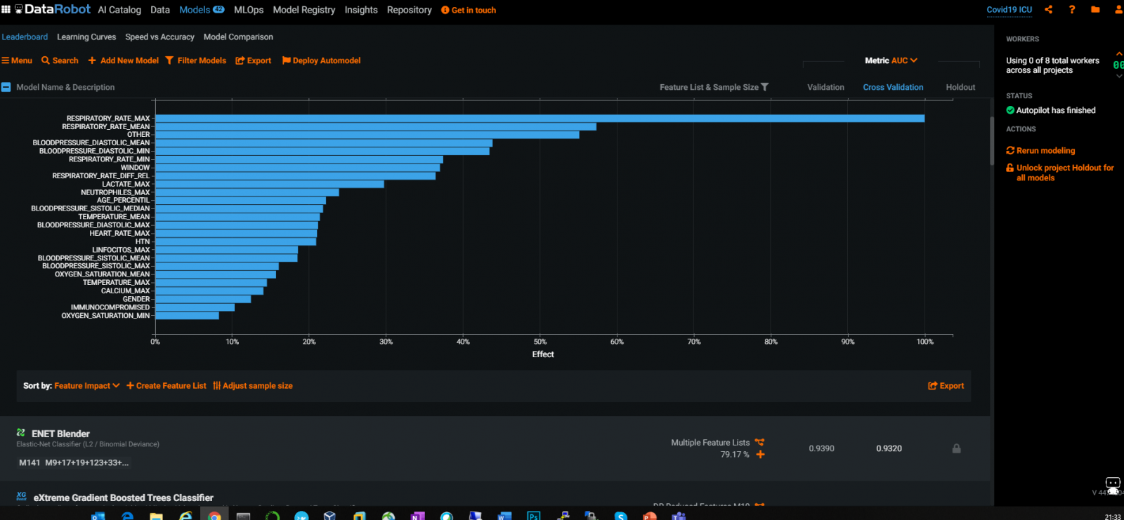
当然ながら、上記のDataRobotグラフから、さまざまなRespiratoryRate値とBloodPressure値がICU入室に最も関連性の高い特徴量であることがわかります。
特徴量の選択 - 最終選択
この記事では、簡単な実験を行い、LightGBMによる特徴量の選択が実際にほんの少し良い結果を出したことに気づいたので、この選択方法のみを使用することにします。
df_selected_columns = embeded_lgb_feature # better than ensembled selectiondataS = pd.concat([idf[df_selected_columns],idf['ICU'], df_cat['WINDOW']],1) dataS.ICU.value_counts() print(dataS.shape)
(1925, 58)
58個の特徴量が選択されていることがわかります。多すぎず、少なからず、この特定のシングルターゲット二項分類問題には適切な量だと言えます。
データの不均衡
plt.figure(figsize=(10,5))
count = sns.countplot(x = "ICU",data=data)
count.set_xticklabels(["Not Admitted","Admitted"])
plt.xlabel("ICU Admission")
plt.ylabel("Patient Count")
plt.show()
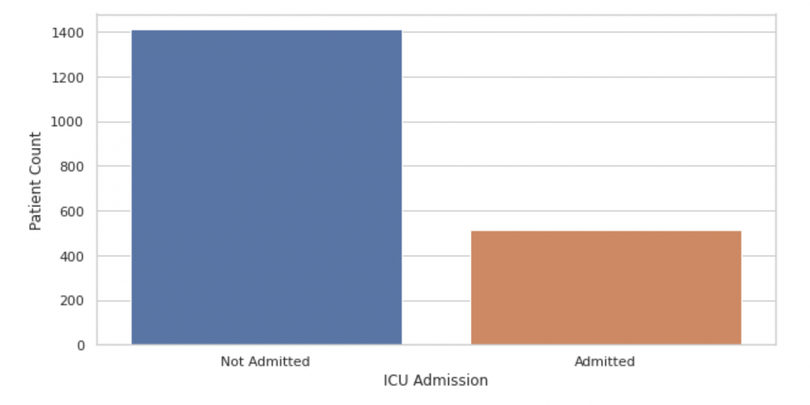
これはデータが不均衡であることを示し、ICUに入室したというレコードは26%のみです。 これは結果に影響を及ぼすため、SMOTEなどの通常のデータ均衡化アプローチを考えられます。
ここでは、他のあらゆる種類のEDAを試し、それに応じてさまざまなデータ分布を理解することができます。
基本的なLRトレーニングを実行する
Kaggleサイトには、独自の特徴量カラムの選択に基づいて素早く実行できる優れた簡易トレーニングノートブックがいくつかあります。 とりあえず、トレーニングパイプラインのLR分類器をさっと実行することから始めましょう。
data2 = pd.concat([idf[df_selected_columns],idf['ICU'], df_cat['WINDOW']],1)
data2.AGE_ABOVE65 = data2.AGE_ABOVE65.astype(int) data2.ICU = data2.ICU.astype(int) X2 = data2.drop("ICU",1) y2 = data2.ICUfrom sklearn.preprocessing import LabelEncoder label_encoder = LabelEncoder() X2.WINDOW = label_encoder.fit_transform(np.array(X2["WINDOW"].astype(str)).reshape((-1,)))
confusion_matrix2 = pd.crosstab(y2_test, y2_hat, rownames=['Actual'], colnames=['Predicted']) sns.heatmap(confusion_matrix2, annot=True, fmt = 'g', cmap = 'Reds') print("ORIGINAL") print(classification_report(y_test, y_hat)) print("AUC = ",roc_auc_score(y_test, y_hat),'\n\n') print("LABEL ENCODING") print(classification_report(y2_test, y2_hat)) print("AUC = ",roc_auc_score(y2_test, y2_hat)) y2hat_probs = LR.predict_proba(X2_test) y2hat_probs = y2hat_probs[:, 1] fpr2, tpr2, _ = roc_curve(y2_test, y2hat_probs) plt.figure(figsize=(10,7)) plt.plot([0, 1], [0, 1], 'k--') plt.plot(fpr, tpr, label="Base") plt.plot(fpr2,tpr2,label="Label Encoded") plt.xlabel('False positive rate') plt.ylabel('True positive rate') plt.title('ROC curve') plt.legend(loc="best") plt.show()
ORIGINAL precision recall f1-score support 0 0.88 0.94 0.91 171 1 0.76 0.57 0.65 54 accuracy 0.85 225 macro avg 0.82 0.76 0.78 225 weighted avg 0.85 0.85 0.85 225 AUC = 0.7577972709551657 LABEL ENCODING precision recall f1-score support 0 0.88 0.93 0.90 171 1 0.73 0.59 0.65 54 accuracy 0.85 225 macro avg 0.80 0.76 0.78 225 weighted avg 0.84 0.85 0.84 225 AUC = 0.7612085769980507
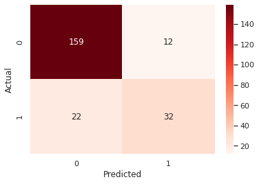
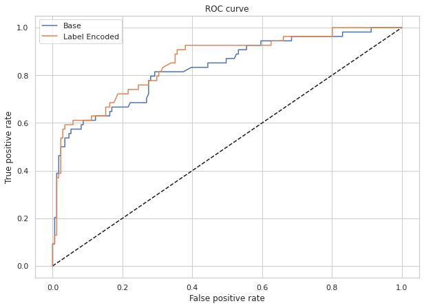
85%の精度でAUC 76%を達成しているようですが、ICU入院のRecallは59%のみで、偽陰性が多すぎるようです。 それは確かに理想的ではありません。患者のレコードに対して実際のICUリスクを見落とすわけにはいきません。 そこで、すべての後続のタスクでは、うまく行けばある程度均衡のとれた全体的精度でFNを下げてRecallレートを引き上げる方法に目標を定めることにします。
前のセクションでは、不均衡データについて触れました。最初の直感は、テストセットを層別化(Stratify)し、SMOTEしてより均衡のとれたデータセットを作成することです。
#テストデータを層別化し、TrainデータとTestデータの比率が同じ1:0になるようにする X3_train,X3_test,y3_train,y3_test = train_test_split(X2,y2,test_size=225/1925,random_state=42, stratify = y2, shuffle = True) <span> </span>train and predict
LR.fit(X3_train,y3_train) y3_hat = LR.predict(X3_test)
#データをSMOTEし、ICU 1:0を均衡のとれた分布にする from imblearn.over_sampling import SMOTE sm = SMOTE(random_state = 42) X_train_res, y_train_res = sm.fit_sample(X3_train,y3_train.ravel()) LR.fit(X_train_res, y_train_res) y_res_hat = LR.predict(X3_test)
#混同行列などをもう一度描画する confusion_matrix3 = pd.crosstab(y3_test, y_res_hat, rownames=['Actual'], colnames=['Predicted']) sns.heatmap(confusion_matrix3, annot=True, fmt = 'g', cmap="YlOrBr") print("LABEL ENCODING + STRATIFY") print(classification_report(y3_test, y3_hat)) print("AUC = ",roc_auc_score(y3_test, y3_hat),'\n\n') print("SMOTE") print(classification_report(y3_test, y_res_hat)) print("AUC = ",roc_auc_score(y3_test, y_res_hat)) y_res_hat_probs = LR.predict_proba(X3_test) y_res_hat_probs = y_res_hat_probs[:, 1] fpr_res, tpr_res, _ = roc_curve(y3_test, y_res_hat_probs) plt.figure(figsize=(10,10))
#前のようにROC曲線をプロットする
LABEL ENCODING + STRATIFY precision recall f1-score support 0 0.87 0.99 0.92 165 1 0.95 0.58 0.72 60 accuracy 0.88 225 macro avg 0.91 0.79 0.82 225 weighted avg 0.89 0.88 0.87 225 AUC = 0.7856060606060606 SMOTE precision recall f1-score support 0 0.91 0.88 0.89 165 1 0.69 0.75 0.72 60 accuracy 0.84 225 macro avg 0.80 0.81 0.81 225 weighted avg 0.85 0.84 0.85 225 AUC = 0.8143939393939393
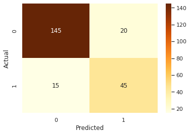
したがって、データのSTRATIFY処理とSMOTE処理はRecallを0.59から 0.75、全体的な精度を0.84に改善しているようです。
従来型MLのデータ処理の大半がいつも通り完了したので、このケースの最善のモデルが何であるかを知りたいと思います。それらはもっと優れているのでしょうか。また、比較的包括的な比較を試みることができるでしょうか。
さまざまなモデルのトレーニング比較を実行する
一般的に使用されているMLアルゴリズムを評価し、箱ひげ図によって、結果の比較ダッシュボードを生成してみましょう。
# アルゴリズムを比較 from matplotlib import pyplot from sklearn.model_selection import train_test_split from sklearn.model_selection import cross_val_score from sklearn.model_selection import StratifiedKFold from sklearn.linear_model import LogisticRegression from sklearn.tree import DecisionTreeClassifier from sklearn.neighbors import KNeighborsClassifier from sklearn.discriminant_analysis import LinearDiscriminantAnalysis from sklearn.naive_bayes import GaussianNB from sklearn.svm import SVC #ランダムフォレストモデルをインポートする from sklearn.ensemble import RandomForestClassifier from xgboost import XGBClassifier
# アルゴリズムを合わせてリストする models = [] models.append(('LR', <strong>LogisticRegression</strong>(solver='liblinear', multi_class='ovr'))) models.append(('LDA', LinearDiscriminantAnalysis())) models.append(('KNN', <strong>KNeighborsClassifier</strong>())) models.append(('CART', <strong>DecisionTreeClassifier</strong>())) models.append(('NB', <strong>GaussianNB</strong>())) models.append(('SVM', <strong>SVC</strong>(gamma='auto'))) models.append(('RF', <strong>RandomForestClassifier</strong>(n_estimators=100))) models.append(('XGB', <strong>XGBClassifier</strong>())) #clf = XGBClassifier()# 代わりに各モデルを評価する results = [] names = [] for name, model in models: kfold = StratifiedKFold(n_splits=10, random_state=1) cv_results = cross_val_score(model, X_train_res, y_train_res, cv=kfold, scoring='f1') ## accuracy, precision,recall results.append(cv_results) names.append(name) print('%s: %f (%f)' % (name, cv_results.mean(), cv_results.std()))
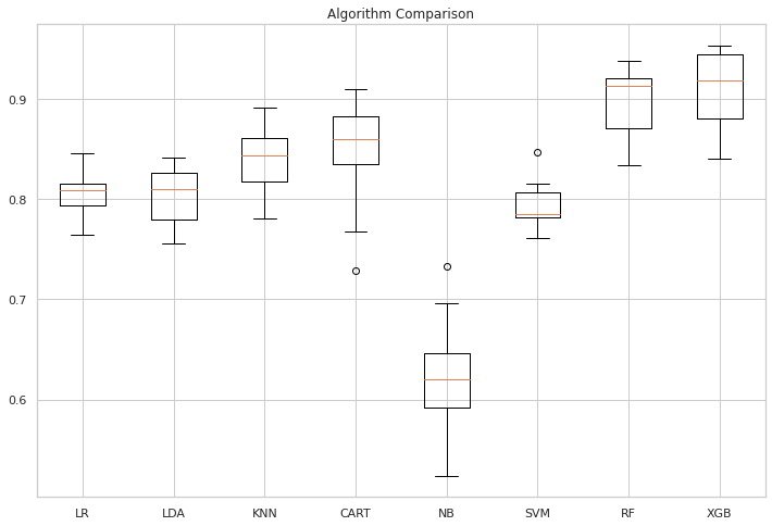
# すべてのモデルのパフォーマンスを比較する。 質問 - それに関する統合アイテムを見たいですか? pyplot.figure(4, figsize=(12, 8)) pyplot.boxplot(results, labels=names) pyplot.title('Algorithm Comparison') pyplot.show()LR: 0.805390 (0.021905) LDA: 0.803804 (0.027671) KNN: 0.841824 (0.032945) CART: 0.845596 (0.053828) NB: 0.622540 (0.060390) SVM: 0.793754 (0.023050) RF: 0.896222 (0.033732) XGB: 0.907529 (0.040693)
上記は、XGB分類子とランダムフォレスト分類子に他のモデルよりも優れたF1スコアがあるように見えます。
同じセットの正規化されたテストデータで実際のテスト結果を比較して見ましょう。
import time from pandas import read_csv from sklearn.model_selection import train_test_split from sklearn.metrics import classification_report from sklearn.metrics import confusion_matrix from sklearn.metrics import accuracy_score from sklearn.svm import SVC
for name, model in models: print(name + ':\n\r') start = time.clock() model.fit(X_train_res, y_train_res) print("Train time for ", model, " ", time.clock() - start) predictions = model.predict(X3_test) #(X_validation) # Evaluate predictions print(accuracy_score(y3_test, predictions)) # Y_validation print(confusion_matrix(y3_test, predictions)) print(classification_report(y3_test, predictions))LR: Train time for LogisticRegression(multi_class='ovr', solver='liblinear') 0.02814499999999498 0.8444444444444444 [[145 20] [ 15 45]] precision recall f1-score support 0 0.91 0.88 0.89 165 1 0.69 0.75 0.72 60 accuracy 0.84 225 macro avg 0.80 0.81 0.81 225 weighted avg 0.85 0.84 0.85 225LDA: Train time for LinearDiscriminantAnalysis() 0.2280070000000194 0.8488888888888889 [[147 18] [ 16 44]] precision recall f1-score support 0 0.90 0.89 0.90 165 1 0.71 0.73 0.72 60 accuracy 0.85 225 macro avg 0.81 0.81 0.81 225 weighted avg 0.85 0.85 0.85 225
KNN: Train time for KNeighborsClassifier() 0.13023699999999394 0.8355555555555556 [[145 20] [ 17 43]] precision recall f1-score support 0 0.90 0.88 0.89 165 1 0.68 0.72 0.70 60 accuracy 0.84 225 macro avg 0.79 0.80 0.79 225 weighted avg 0.84 0.84 0.84 225
CART: Train time for DecisionTreeClassifier() 0.32616000000001577 0.8266666666666667 [[147 18] [ 21 39]] precision recall f1-score support 0 0.88 0.89 0.88 165 1 0.68 0.65 0.67 60 accuracy 0.83 225 macro avg 0.78 0.77 0.77 225 weighted avg 0.82 0.83 0.83 225
NB: Train time for GaussianNB() 0.0034229999999979555 0.8355555555555556 [[154 11] [ 26 34]] precision recall f1-score support 0 0.86 0.93 0.89 165 1 0.76 0.57 0.65 60 accuracy 0.84 225 macro avg 0.81 0.75 0.77 225 weighted avg 0.83 0.84 0.83 225
SVM: Train time for SVC(gamma='auto') 0.3596520000000112 0.8977777777777778 [[157 8] [ 15 45]] precision recall f1-score support 0 0.91 0.95 0.93 165 1 0.85 0.75 0.80 60 accuracy 0.90 225 macro avg 0.88 0.85 0.86 225 weighted avg 0.90 0.90 0.90 225
RF: Train time for RandomForestClassifier() 0.50123099999999 0.9066666666666666 [[158 7] [ 14 46]] precision recall f1-score support 0 0.92 0.96 0.94 165 1 0.87 0.77 0.81 60 accuracy 0.91 225 macro avg 0.89 0.86 0.88 225 weighted avg 0.91 0.91 0.90 225
XGB: Train time for XGBClassifier(base_score=0.5, booster='gbtree', colsample_bylevel=1, colsample_bynode=1, colsample_bytree=1, gamma=0, gpu_id=-1, importance_type='gain', interaction_constraints='', learning_rate=0.300000012, max_delta_step=0, max_depth=6, min_child_weight=1, missing=nan, monotone_constraints='()', n_estimators=100, n_jobs=0, num_parallel_tree=1, random_state=0, reg_alpha=0, reg_lambda=1, scale_pos_weight=1, subsample=1, tree_method='exact', validate_parameters=1, verbosity=None) 1.649520999999993 0.8844444444444445 [[155 10] [ 16 44]] precision recall f1-score support 0 0.91 0.94 0.92 165 1 0.81 0.73 0.77 60 accuracy 0.88 225 macro avg 0.86 0.84 0.85 225 weighted avg 0.88 0.88 0.88 225
RFが実際にXGBよりも優れているという結果が出たようです。 XGBが何らかの形で過学習している可能性を示唆しているかもしれません。 RFCの結果はLRよりもわずかに改善されています。
「グリッド検索によるパラメーターチューニング」をさらに行って、選択されたモデルを実行する
では、ランダムフォレスト分類子がここで選ばれたモデルと仮定しましょう。 このモデルにさらにグリッド検索を実行して、結果のパフォーマンスをわずかにでも向上させられるかを確認することができます。
ここでの目標は、患者が遭遇する潜在的なICUリスクの偽陰性を最小限に抑えることで、このケースのRecallを最適化することに変わりはありませんので、「recall_score」を使用して、グリッド検索を再適合させます。 繰り返しますが、上記のテストセットは常に2915件のレコードの約12%に設定されていたため、ここでも10倍の交差検定を使用します。
from sklearn.model_selection import GridSearchCVランダム検索の結果に基づいてパラメーターグリッドを作成する
param_grid = {'bootstrap': [True], 'ccp_alpha': [0.0], 'class_weight': [None], 'criterion': ['gini', 'entropy'], 'max_depth': [None], 'max_features': ['auto', 'log2'],
'max_leaf_nodes': [None], 'max_samples': [None], 'min_impurity_decrease': [0.0], 'min_impurity_split': [None], 'min_samples_leaf': [1, 2, 4], 'min_samples_split': [2, 4], 'min_weight_fraction_leaf': [0.0], 'n_estimators': [100, 125], #'n_jobs': [None], 'oob_score': [False], 'random_state': [None], #'verbose': 0, 'warm_start': [False] }
#混同行列でファインチューニングする from sklearn.metrics import roc_curve, precision_recall_curve, auc, make_scorer, recall_score, accuracy_score, precision_score, confusion_matrix scorers = { 'recall_score': make_scorer(recall_score), 'precision_score': make_scorer(precision_score), 'accuracy_score': make_scorer(accuracy_score) }
# ベースモデルを作成する rfc = RandomForestClassifier()Instantiate the grid search model
grid_search = GridSearchCV(estimator = rfc, param_grid = param_grid, scoring=scorers, refit='recall_score', cv = 10, n_jobs = -1, verbose = 2)
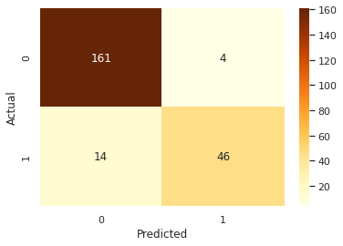
train_features = X_train_resgrid_search.fit(train_features, train_labels)rf_best_grid = grid_search.best_estimator_rf_best_grid.fit(train_features, train_labels) rf_predictions = rf_best_grid.predict(X3_test) print(accuracy_score(y3_test, rf_predictions))
print(confusion_matrix(y3_test, rf_predictions)) print(classification_report(y3_test, rf_predictions))
0.92
[[ 46  14]
[  4 161]]
precision    recall  f1-score   support
0       0.92      0.77      0.84        60
1       0.92      0.98      0.95       165
accuracy                           0.92       225
macro avg       0.92      0.87      0.89       225
weighted avg       0.92      0.92      0.92       225
グリッド検索は、FNを同じに保ちながら、実際に全体的な精度を少し上げることができるという結果が得られました。
AUC比較もプロットしてみましょう。
confusion_matrix4 = pd.crosstab(y3_test, rf_predictions, rownames=['Actual'], colnames=['Predicted']) sns.heatmap(confusion_matrix4, annot=True, fmt = 'g', cmap="YlOrBr")print("LABEL ENCODING + STRATIFY") print(classification_report(y3_test, 1-y3_hat)) print("AUC = ",roc_auc_score(y3_test, 1-y3_hat),'\n\n')print("SMOTE") print(classification_report(y3_test, 1-y_res_hat)) print("AUC = ",roc_auc_score(y3_test, 1-y_res_hat), '\n\n')print("SMOTE + LBG Selected Weights + RF Grid Search") print(classification_report(y3_test, rf_predictions)) print("AUC = ",roc_auc_score(y3_test, rf_predictions), '\n\n\n')
y_res_hat_probs = LR.predict_proba(X3_test) y_res_hat_probs = y_res_hat_probs[:, 1]
predictions_rf_probs = rf_best_grid.predict_proba(X3_test) #(X_validation) predictions_rf_probs = predictions_rf_probs[:, 1]
fpr_res, tpr_res, _ = roc_curve(y3_test, 1-y_res_hat_probs) fpr_rf_res, tpr_rf_res, _ = roc_curve(y3_test, predictions_rf_probs)
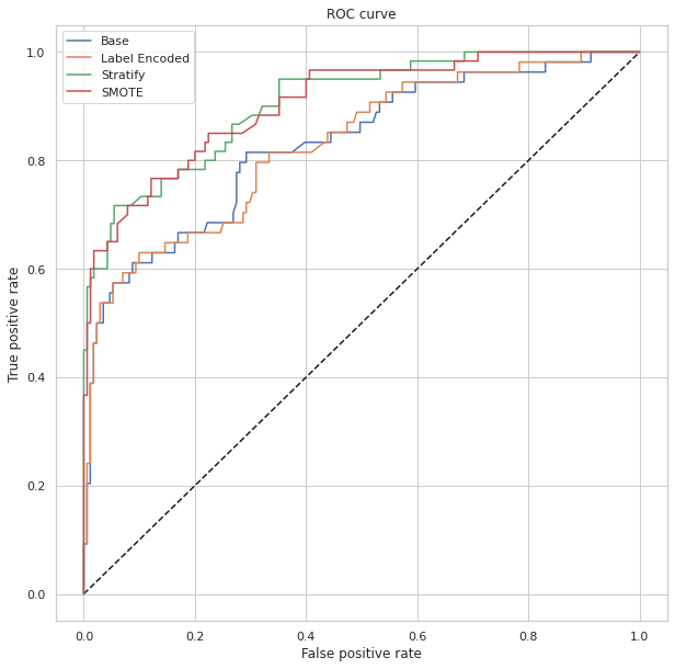
plt.figure(figsize=(10,10)) plt.plot([0, 1], [0, 1], 'k--') plt.plot(fpr, tpr, label="Base") plt.plot(fpr2,tpr2,label="Label Encoded") plt.plot(fpr3,tpr3,label="Stratify") plt.plot(fpr_res,tpr_res,label="SMOTE") plt.plot(fpr_rf_res,tpr_rf_res,label="SMOTE + RF GRID") plt.xlabel('False positive rate') plt.ylabel('True positive rate') plt.title('ROC curve') plt.legend(loc="best") plt.show()
LABEL ENCODING + STRATIFY precision recall f1-score support 0 0.95 0.58 0.72 60 1 0.87 0.99 0.92 165 accuracy 0.88 225 macro avg 0.91 0.79 0.82 225 weighted avg 0.89 0.88 0.87 225 AUC = 0.7856060606060606SMOTE precision recall f1-score support 0 0.69 0.75 0.72 60 1 0.91 0.88 0.89 165 accuracy 0.84 225 macro avg 0.80 0.81 0.81 225 weighted avg 0.85 0.84 0.85 225 AUC = 0.8143939393939394
SMOTE + LBG Selected Weights + RF Grid Search precision recall f1-score support 0 0.92 0.77 0.84 60 1 0.92 0.98 0.95 165 accuracy 0.92 225 macro avg 0.92 0.87 0.89 225 weighted avg 0.92 0.92 0.92 225 AUC = 0.8712121212121211
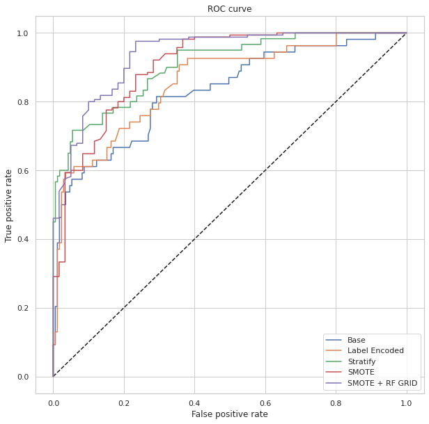
アルゴリズム比較とさらなるグリッド検索の結果、AUCを78%から87%に引き上げることができ、全体の精度は92%、Recallは77%という結果を得られました。
「従来型ML」アプローチのまとめ
では、実際のところこの結果はどうなのでしょうか。 従来型MLアルゴリズムを使った基本的な手動プロセスとしては十分と言えます。 Kaggleコンペティションではどのように見えるでしょうか。 まぁ、リーダーボードには上がらないでしょう。 DataRobotの現在のAutoMLサービスから生のデータセットを実行したところ、最良の結果は、上位43個のモデルを比較したうち、「教師なし学習特徴によるXGBツリー分類子」モデルで、約90%以上相当のAUCを達成すると主張するでしょう。 本当にKaggleに参戦したいのであれば、これが私たちが狙いとする実用的なモデルと言えるでしょう。 最高の結果とモデルの上位リストもGitHubに添付しておきます。 最終的には、ケアサイトに特化した実際のケースについて言えば、この記事の「データとタスク」セクションで述べたように、ある程度カスタマイズされたディープラーニングアプローチにも焦点を当てる必要があると感じています。 もちろん、実際のケースでは、質の高いデータカラムをどこで収集するのかという手前の問題もあるでしょうが。
IntegratedMLアプローチとは
上記では、いわゆる従来型MLと呼ばれるプロセスを説明しました。通常は、データEDA、特徴量エンジニアリング、特徴量の選択、モデルの選択、およびグリッド検索などによるパフォーマンスの最適化が含まれるプロセスです。 これがこのタスクにおいて、今のところ思いつく最も単純なアプローチです。まだモデルのデプロイやサービス管理のライフサイクルについては触れていません。これについては次の記事で、Flask/FlasAPI/IRISを利用して、この基本MLモデルをCovid-19X線画像デモサービススタックにデプロイする方法を探りながら、説明したいと思います。
IRISにはIntegratedMLが組み込まれており、強力なAutoMLオプションの洗練されたSQLラッパーとして用意されています。 パート2では、ビジネスのメリットとして同等のML結果を引き出しながら、特徴量の選択、モデルの選択、パフォーマンスの最適化などを行わずに済むように、上記のタスクを大幅に単純化したプロセスで達成する方法を調べます。
以上です。同じデータでintegratedMLのクイックランをこの記事に追加するには、10分メモとしては長すぎてしまうため、次のパート2の記事で話すことにします。